HUBLE METHODS
Quality control (QC) protocol for Genome Wide Association Study (GWAS) data
Introduction
This HubLE method provides a short protocol for performing quality control in Genome-Wide Association Studies (GWAS) prior to testing for association with the trait of interest.
Materials
- Genotyped data from Genome Wide Association Study (GWAS)
- Computer (hardware)
- UNIX/Linux software
- PLINK software (http://zzz.bwh.harvard.edu/plink/download.shtml [Tip No. 1].
- Human reference 1000 Genomes project
(http://www.1000genomes.org/)
Methods [Update]
- File preparation. Create binary files .bed, .bim, .fam in PLINK [Tip No. 2] using the following script on the input file (for e.g. “data”; where in this particular example, PLINK will expect the files data.ped and data.map as input): PLINK –file data –make-bed –out mydata
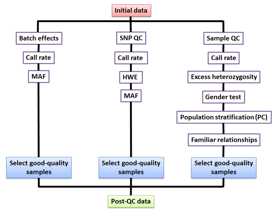
- SNP filtering is based on ( Fig. 1):
- Call rate: SNPs that show low genotyping efficiency are removed using the command: plink –bfile mydata –geno 0.01 –make-bed –out mydata_geno
- Minor allele frequency (MAF) [Tip No. 3]. Rare alleles are removed using the following: plink –bfile mydata –maf 0.01 –make-bed –out mydata_maf
- Hardy-Weinberg equilibrium (HWE). Markers that fail Hardy-Weinberg equilibrium are removed using the script: plink –bfile mydata –hwe 0.000001 –make-bed –out mydata_hwe
3. Individual/sample-level filtering is based on ( Fig. 1):
- Call rate: individuals with an excess of missing genotype data can be removed as follows: plink –bfile mydata –mind 0.01 –make-bed –out mydata_missing and a summary of missingness in a sample can be obtained by the command: plink –bfile mydata –missing –outmydata_missing
- Heterozygosity: This filters out individuals with excess or reduced heterozygosity by assessing observed (O) and expected (E) counts of heterozygous SNPs (genotypes) in an individual using the following command: plink–bfile mydata–het–out mydata_het [Tip No. 5].
- Gender estimation: PLINK uses data from chromosome X to determine sex by using the command:plink –bfile mydata –check-sex –out mydata_sex [Tip No. 6].
- Population stratification: or presence of multiple subpopulations (different ethnic backgrounds) is corrected by a principal component analysis (PCA). 1000Genomes can provide a reference panel to compare the populations. To create a relatedness matrix, use pairwise IBS (identity-by-state) distances as follows: The threshold 10-6 for HWE is commonly used in GWAS. [Tip No. 4]. plink –bfile mydata –genome –out mydata_IBS Group differences are obtained using script: plink –bfile mydata –read-genome plink.genome –ibs-test
- Group relatedness in samples can be visualised by: plink –file mydata –read-genome plink.genome –cluster –mds-plot 4
- Plotting each principal component against the other will offer a scatter plot with a point per individual [Tip No. 7].
- Relatedness or cryptic familial relationships: This indicates the strength of genetic relatedness in a pair of individuals [Tip No. 8].
IBS matrix can also to detect identity by descent (IBD) information between pairs of samples using the –genome command as described above.
To avoid strong correlations between SNPs due to inbreeding populations, perform LD pruning [Tip No. 9] to select a subset of SNPs that are not or weakly correlated with each other using an r2 threshold of 0.2 as follows: plink –bfile mydata –indep-pairwise 50 5 0.2 –out mydata_IBS
This creates a list of SNPs (mydata_IBS.prune.in) to be retained in the analysis and another (mydata_IBS.prune.out) for those to be excluded.
Tips [Update]
PLINK is a user-friendly and freely available software. The scripts mentioned in this protocol have been extracted from the PLINK tutorial, that can be found in full at: http://zzz.bwh.harvard.edu/plink/tutorial.shtml. There are alternative tools for quality control which also allow more plasticity in the scripts, like R software. The R package EasyQC1 contains pre-made scripts and needed reference files to perform GWAS QC on genotyped data.
- PLINK supports .ped (linkage-style pedigree file) and .map (SNP location) files, but the binary files save time and space. PLINK .bed file contains binary version of the genotype data. Pedigree information is stored in .fam file and .bim contains SNP location data.
- Minor allele frequency threshold depends on the size of the study and the effect size of the change(s). Large studies (N =100,000 or more) tend to use MAF threshold = 0.01, whilst smaller sized studies set the MAF threshold = 0.05. Rare SNPs in small populations are prone to genotyping errors. PLINK uses MAF=0.01 as default value.
- Deviations from HWE commonly indicate genotyping errors in GWAS but may also result from population substructure or evolutionary selection. For case-control studies, the HWE filtering is only performed in the controls, since true associations in cases usually violate this rule.
- Individuals with extreme values (±3 standard deviation from the samples’ heterozygosity mean) are considered outliers and should be removed from the data set2. Excess values for genotyped SNPs in an individual indicate possible sample DNA contamination and reduced values may indicate possible inbreeding or population substructure.
- Discrepancies between sex determined in input pedigree files and sex obtained by X-chromosome analyses indicates a possible sample mix-up. A threshold value of X chromosome homozygosity estimate (F) > 0.8 for males and < 0.2 for females is generally used2. Sex discrepancy can also arise owing to chromosomal abnormalities (i.e. Turner or Klinefelter syndrome). A visual tool to inspect causes of gender mismatch is the GenomeStudio software (Illumina)3.
- Since allele frequencies can differ between subpopulations, this stratification can result in spurious associations and indeed masking of true associations. The Z-score is calculated based on the sample mean and variance, and samples with extreme values, usually deviating ± 4 standard deviation units, are considered outliers and should be removed3.
- GWAS assumes that all study participants are unrelated. As a result, including those with a strong genetic relation in the GWAS may lead to biased estimations of SNP effects. An IBD kinship coefficient (PI_HAT) > 0.1 suggests either strong relatedness or duplication amongst the sample pair under test unless there is sample DNA contamination prior to genotyping4. One sample per pair will then be excluded from analysis (unless a software that can account and adjust for family structure is used). The sample selected for exclusion is usually of low genotype call rate or one that minimises sample number loss or phenotype availability and interest.
- By specifying a linkage disequilibrium (LD) threshold (for e.g. 0.2), PLINK uses the level of LD between SNPs located within a specific region of chromosome and selects a set of correlated SNPs. This LD pruning reduces redundancy in the data and influence of chromosomal artefacts4, thus advisable prior to performing IBS and PCA analysis.
- Additional tip(s): It is also a good practice to test for batch effects when combining samples from different laboratories and/or different genotyping platforms. A simple approach is to test differences in average MAF and call rate for the same SNP across all the plates5. Any batch related significance can also be tested by testing one plate or batch against other plates/batches in the same assay/study5. This involves coding one plate as cases and remainder as controls. A simple association test is then performed to detect any deviation from expected uniform distribution of p values. Any discrepancy can be treated in same way as population stratification.
References [Update]
- EasyQC.
Marees A.T., de Kluiver H., Stringer S., Vorspan F., Curis E., Marie-Claire C., Derks E.M. A tutorial on conducting genome-wide association studies: Quality control and statistical analysis. International Journal of Methods in Psychiatric Research, 2018; 27(2):e1608.
- Alonso N., Lucas G.and Hysi P. Big data challenges in bone research: GWAS and NGS. Bonekey Reports., 2015; 11; 4:635.
- Reed E., Nunez S., Kulp D., Qian J., Reilly M. P., & Foulkes, A. S. A guide to genome‐wide association analysis and post‐analytic interrogation. Statistics in Medicine, 2015; 34(28), 3769–3792.
- Turner S., Armstrong L.L., Bradford Y., Carlson C.S., Crawford D.C., Crenshaw A.T et al. Quality control procedures for genome-wide association studies. Current Protocols in Human Genetics, 2011; Chapter 1:Unit1.19.

Sachin Wani, PhD
Rheumatology and Bone Disease Unit, IGMM, University of Edinburgh, Edinburgh, UK.
Email: swani@exseed.ed.ac.uk

Nerea Alonso, PhD
Rheumatology and Bone Disease Unit, IGMM, University of Edinburgh, Edinburgh, UK.
Email: n.alonso@ed.ac.uk


